Text Classification and Bayes' Theorem
Some evenings, you will find me engaged in a fierce, albeit friendly, competition Six Card Golf with my family. Admittedly, repetitive play has dulled the excitement over the past several months. My favorite part is anticipating an opponent becoming distracted and giving up a card that completes a competitor’s row!
Six Card Golf
Golf is about conditional probability. Players start with their cards face down and have to make a choice each turn: reveal a card, swap with a known deck card, or swap with an unknown deck card. The trick is knowing what your opponents have already revealed because the goal of the game is to match rows by rank to cancel them out. Just like golf, each unmatched card per row adds up at the end. The person with the biggest score after 9 “holes” is known as the “goat” (not to be mistaken with the “G.O.A.T.”).
We combine two decks (with jokers) for seven players, so the total number of cards is 108. You might not think there’s a way to strategize before the game begins, but let’s focus on what we know:
- The chances of pulling a king (zero points) or an ace (one point) is $\frac{16}{108}$, or $14.81\%$.
- The chances of pulling the best card in the game (joker) is $\frac{4}{108}$, or $3.70\%$.
- The chances of pulling three cards of the same rank and immediately having a matched row is:
The last bullet is found by considering how we could choose three cards from the deck ${108 \choose 3}$, how many ways we could draw three cards of the same rank ${8 \choose 3}$ for any of the 13 different ranks, and finally dividing.
Decision-making
We’ve determined the chances associated with the initial six face-down cards you’re dealt with and the chances of drawing a favorable card, but as the game progresses, your strategy may change. If you have a row of two fives and hope to eventually draw one more, the cards your opponents have revealed mean a great deal (no pun intended). For instance, if my grandma has two fives and my sister has two, my chances of drawing a five are greatly diminished. Two more fives would be left in the deck or among your remaining face-down cards.
The probabilities we calculated earlier based on the chances of a particular card appearing is known as a priori knowledge. Knowing my grandma and sister have each two fives revealed midway through the game is known as a posteriori knowledge.
The Law of Total Probability
If you know why I named my blog “Universal Set” you may already understand it’s a reference to set theory. If not, you should read my about page. I want to first introduce the concept of a partition. A partition of a set is a collection of non-empty subsets $(i)$ that are mutually exclusive $(ii)$ and collectively exhaustive $(iii)$. (Goldberg, 1987)
\[\begin{align*} \text{(i)}\quad & E_j \subseteq E & (j = 1, 2, \ldots, n) \\ \text{(ii)}\quad & E_j \cap E_k = \emptyset & (j = 1, 2, \ldots, n, k = 1, 2, \ldots, n, j \ne k) \\ \text{(iii)}\quad & E_1 \cup E_2 \cup \ldots \cup E_n = E \end{align*}\]For example, sets $F$ and $\overline{F}$ form partition $\set{F, \overline{F}}$.
Let events $\set{E_1, E_2, \ldots, E_n}$ be a partition of sample space $S$ and suppose each event have a nonzero probability. Let’s find the probability of event $E$ given a partition of these $E_j$ events.
\[P(E) = \sum_{j=1}^{n} P(E_j)P(E \mid E_j)\]The total probability of event $E$ is the weighted sum of the conditional probabilities of E occurring given each partitioning events $E_j$. The weights are the probabilities $E_j$ themselves.
Let’s shuffle our Golf deck of 108 cards and consider the likelihood that a joker is next to a king. We must consider three cases: the joker is at the deck’s top $(E_1)$, end $(E_2)$, or middle $(E_3)$. If the joker is in the middle, the king could be before or after it. Notice $\set{E_1, E_2, E_3}$ form a partition of sample space $S$ which is all possible orderings of a 108-card deck.
\[\begin{align*} \quad & P(E_1) = P(E_2) = \frac{1}{27}, & P(E_3) = \frac{25}{27},\\ \quad & P(E \mid E_1) = P(E \mid E_2) = \frac{8}{107}, & P(E \mid E_3) = \frac{16}{107}\\ \end{align*}\]$P(E \mid E_1)$ is found by knowing there are 8 kings in this combined deck and we consider the joker is on top/bottom which means 107 cards remain. When the joker is in the middle, a king could be neighboring above or below it which gives us the conditional probability of $\frac{16}{107}$. We then use the law of total probability to discover the probability of event $E$
\[\begin{align*} P(E) &= (\frac{1}{27})(\frac{8}{107}) + (\frac{1}{27})(\frac{8}{107}) + (\frac{25}{27})(\frac{16}{107})\\ P(E) &= \frac{416}{2889} \approx 14.4\% \end{align*}\]Bayes’ Theorem
Since we now understand the law of total probability, let’s turn to Bayes’s Theorem.
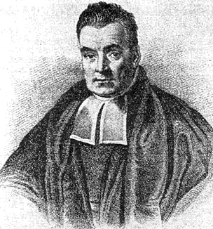
Thomas Bayes was an English minster and statistician whose work was published posthumously by the Royal Society of London in 1763. His theorem reveals the probability of a hypothesis $E_k$ given the occurrence of some evidence $E$ – known as posterior probability. If $E$ has a nonzero probability and $(1 \leq k \leq n)$ we have Bayes’ Theorem
\[P(E_k \mid E) = \frac{P(E_k)P(E \mid E_k)}{\sum_{j=1}^{n} P(E_j)P(E \mid E_j)} = \frac{P(E_k)P(E \mid E_k)}{P(E)}\]This can be applied to sequential events where additional information later acquired impacts the initial probability. Remember, Bayes’ Theorem is only applicable if $\set{E_1, E_2, \ldots, E_n}$ is a partition of the sample space for the experiment.
Naïve Bayes Algorithm
The process of deriving useful information from a raw text string is known as Natural Language Processing (NLP). The Naïve Bayes algorithm is based on Bayes’ Theorem and is particularly optimized for count vectorization for text data.
Let’s start with a problem I think is fascinating and worth solving: how can we determine if a text string is a suggestion? Consider we have a list of a hundred various text strings with labels:
| text | label |
|---|---|
| Consider trying a new approach to solve this problem | 1 |
| The sky is clear and blue today | 0 |
| Maybe exploring a different genre would be interesting | 1 |
| This coffee tastes amazing | 0 |
We have 66 suggestions and 33 non-suggestions. Let’s break up all word occurrences from either category and consider how often they appear in each. I will make up this data to simplify the problem and help demonstrate Bayes’ Theorem.
- $P(S) = 0.67$ the text is a suggestion
- $P(S’) = 0.33$ the text is not a suggestion
- $P(\text{“should”} \mid S) = 0.25$ the word “should” appears in $\frac{3}{4}$ of the suggestion dataset
- $P(\text{“should”} \mid \overline{S}) = 0.05$ the word “should” appears in $\frac{3}{4}$ of the non-suggestion dataset
Given these probabilities, what if we receive a string that says, “Somebody should throw that away”? Let’s use Bayes’ Theorem to compute the likelihood this is a suggestion:
\[\begin{align*} P(S \mid \text{input}) &= \frac{P(\text{input})P(\text{input} \mid S)}{P(S)} = \frac{0.25}{0.67} \approx 0.37\\ P(\overline{S} \mid \text{input}) &= \frac{P(\text{input})P(\text{input} \mid \overline{S})}{P(\overline{S})} = \frac{0.05}{0.33} \approx 0.15 \end{align*}\]Since $0.37 \gt 0.15$ this text will be classified as a suggestion.
The Naïve Bayes algorithm models the probability of belonging to $k$ class ($C_k$) given a vector of $n$ features ($x_n$). The classes for suggestion detection are “suggestion” and “non-suggestion”. The features consist of a collection of measurable properties such as an email containing certain words.
\[P(C_k \mid E) = \frac{P(C_k)P(x \mid C_k)}{P(x)} = \frac{P(C_k, x_1, \ldots, x_n)}{P(x)}\]The “naïve” here refers to the assumption that feature pairs are mutually independent. Linguistically, words are dependent when used in a comprehensible sentence, but this assumption performs well when we treat language as a simple bag of words!
Training a Classifier
This small project aims to successfully classify an arbitrary string as “suggestion” or “non-suggestion” via supervised learning. To kick off this project, I will use a unique method of obtaining fake labeled data by running my synthetic-data-generator script from an earlier project, which will call the OpenAI API, and create 100 labeled rows of suggestions and non-suggestions. Clone my notebooks repo if you wish to follow along!
Running the script provided me with over a hundred pairs such as this:
1
2
3
4
["Consider trying a new approach to solve this problem", 1]
["The sky is clear and blue today", 0]
["Maybe exploring a different genre would be interesting", 1]
["This coffee tastes amazing", 0]
As I mentioned before, this algorithm treats each word independently and determines the frequency of a word per class. To briefly demonstrate what this looks like behind the scenes, we’ll import CountVectorizer to extract the feature names of all our suggestions. I want to ignore the most common stop words in the English language as they will be inconsequential.
1
2
3
4
5
6
7
8
9
# Create list of suggestion features
suggestions = [item[0] for item in data if item[1] == 1]

count_vect = CountVectorizer(stop_words='english')
matrix = count_vect.fit_transform(suggestions)
freq = zip(count_vect.get_feature_names_out(), matrix.sum(axis=0).tolist()[0])

# Sort by frequency and print the top 3
sorted(freq, key=lambda x: -x[1])[:3]
The top three most frequent words are what you may expect given suggestions imply change.
1
[('consider', 10), ('new', 9), ('different', 6)]
Now, if we want to evaluate our model we should split our features and labels into training and testing data. Adding the random state parameter makes this split repeatable.
1
X_train, X_test, y_train, y_test = train_test_split(texts, labels, test_size=0.33, random_state=42)
Next, let’s vectorize the features by word and use the training data to fit a Multinomial Naïve Bayes classifier. A Multinomial Naïve Bayes classifier is better suited for datasets with discrete labels (e.g. text classification).
1
2
3
4
5
6
vectorizer = CountVectorizer()
X_train = vectorizer.fit_transform(X_train)
X_test = vectorizer.transform(X_test)

model = MultinomialNB()
model.fit(X_train, y_train)
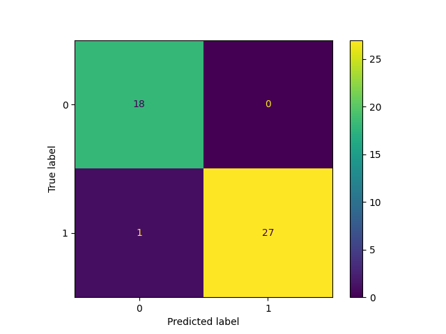
Finally, let’s generate a performance report based on model accuracy and plot a confusion matrix for running the model against the test dataset.
1
2
3
4
5
6
7
8
9
10
11
12
13
14
15
16
17
y_pred = model.predict(X_test)

cm = confusion_matrix(y_test, y_pred, labels=[0,1])

print(classification_report(y_test, y_pred, labels=[0,1]))
disp = ConfusionMatrixDisplay(confusion_matrix=cm, display_labels=[0,1])
disp.plot()


              precision    recall  f1-score   support

           0       0.95      1.00      0.97        18
           1       1.00      0.96      0.98        28

    accuracy                           0.98        46
   macro avg       0.97      0.98      0.98        46
weighted avg       0.98      0.98      0.98        46
Out of the randomly selected 46 features only one label was predicted to be “non-suggestion” when it really was a suggestion. This report shows an accuracy of about 98%. Keep in mind this was a simple experiment on synthetic data. Models are only as good as your data!
Theory and Practice
I hope this post has demonstrated how mathematical principles can be applied to solve challenging problems. Discovering concepts of probability theory will enrich your understanding of machine learning techniques.
If you are a technical professional, I encourage you to revisit your old probability & statistics, linear algebra, and multivariate calculus textbooks because despite the false theory-practice dichotomy: all good theories work in practice. Behind the mystique of every Python library is matrix multiplication, convolution, and gradient descent.
Reference
- Goldberg, S. (1987). Probability: An Introduction. Dover.


